
 RSMUS.com
As technology professionals, we are constantly looking for new ways to connect different technologies and streamline processes. Recently, we became curious as to how Power BI may be able to display an interactive predictive model that we had tested, trained, and created in R. For those not familiar with the technologies, R-studio is a powerful tool for code-based data transformation, cleansing, and predictive modeling. On the other hand, Power BI allows an end-user to create reports and visualizations code-free based on datasets. For a copy of the .pbix file, please contact nicole.anderson2@rsmus.com.
Through research and development, we were able to successfully create an interactive and dynamic interface in Power BI that displays the results of a model in real-time. This process can be used to show predictions from linear regression models, whether that be sales, production numbers, and the likelihood of something occurring. This process allows people with lower technical skills to have predictive modeling at their fingertips.
You may or may not be aware that Power BI has some predictive visualization abilities, but this process has the benefit of training and testing of a model and displaying it to end-users. One thing to note is that while developing this process, we found that there were some storage limitations for the connection of the Power BI to the model in R. For this reason, I’ve limited the dataset to a random sample of 50 records. If you’re interested to see how this process works or want to try it out yourself, read ahead on the specific steps and configurations to make this possible.
Configure predictive visualization abilities
1. Open R-Studio. Define the data frame and define the linear model:
df = read.csv("SampleAdmitData.csv")
library(dplyr)
df= sample_n(df, 50)
model = lm(admit ~ gre + gpa + rank, df)
2. Then, run the following script in R. Make sure to change the location string to somewhere on your local drive. This defines the location where the model will be saved so that it can be pulled in by Power BI.
project_folder <- "~/Admissions_Model/"
finalfit <- model
saveRDS(model, file = paste0(project_folder, "admission_model.rds"))
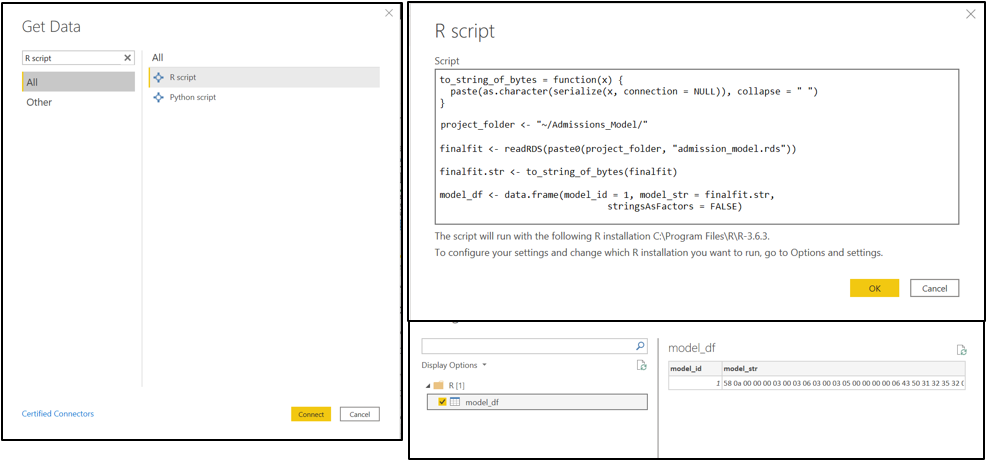
3. Now, open Power BI Desktop and select ‘Get Data’. Search ‘R Script’ and select it. Use the code below to pull in a serialized version of the model. It comes through as a long string of random characters.
to_string_of_bytes = function(x) {
paste(as.character(serialize(x, connection = NULL)), collapse = " ")
}
project_folder <-
"~/Admissions_Model/"
finalfit <- readRDS(paste0(project_folder, "admission_model.rds"))
finalfit.str <- to_string_of_bytes(finalfit)
model_df <- data.frame(model_id = 1, model_str = finalfit.str,
stringsAsFactors = FALSE)
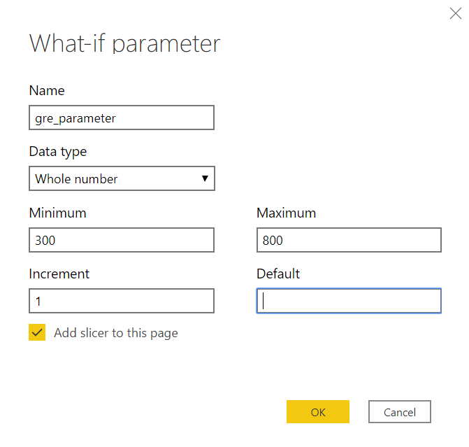
4. The next step is to create the parameters and sliders that allow for the end visual to be dynamic. Navigate to the ‘Modeling’ tab in Power BI. For all numeric variables, select ‘New Parameter’. Minimum and Maximum values were found using the summary() function in R. Input the requirements to create a parameter.
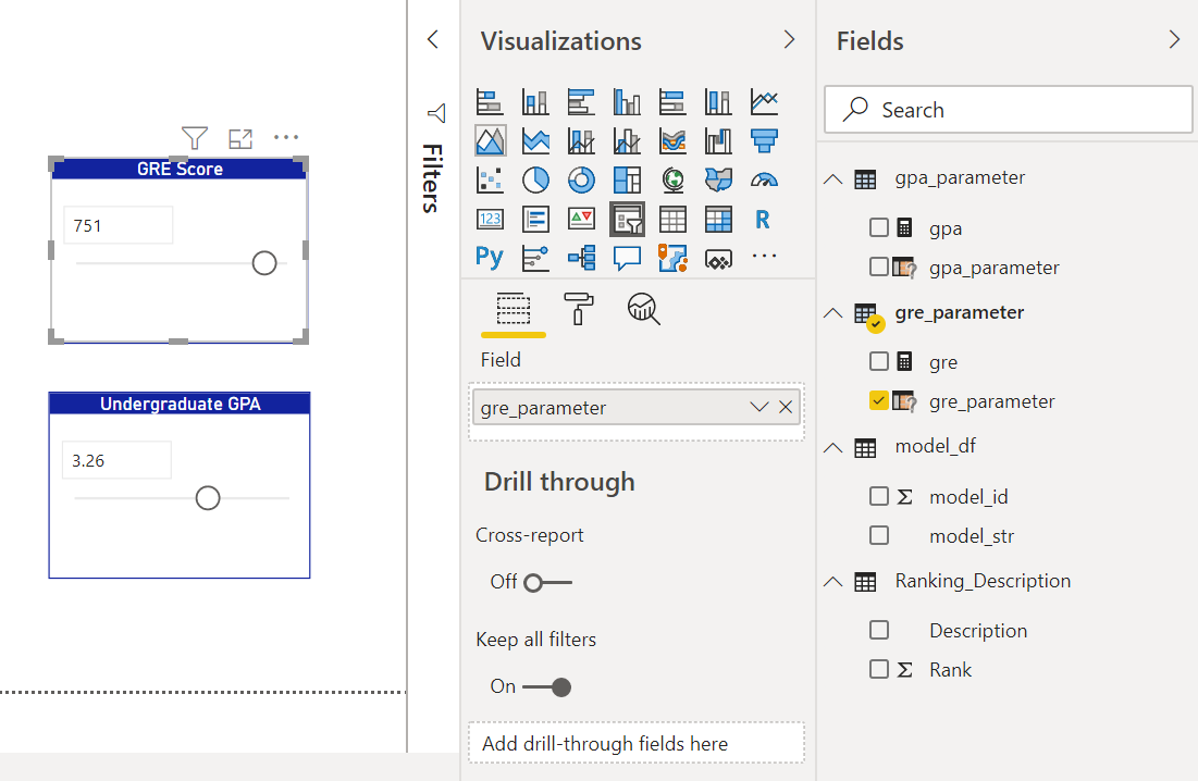
Under each parameter on the right-hand side, there is a measure and a parameter field. The parameter field ties to the slicer visualization, while the measure will tie to the R Script visualization.
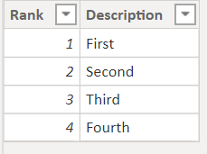
5. For categorical variables, a reference table will need to be created to ensure that an end-user can select the descriptive category, rather than a number, within the slicer visualization.
- Select ‘Enter data’ on the Home tab of Power BI. Enter the respective numbers associated with each category. For example, with ‘Rank’ variable:

- Then, place the ‘Description’ column in a Slicer visualization, similar to the parameters created for numeric variables.
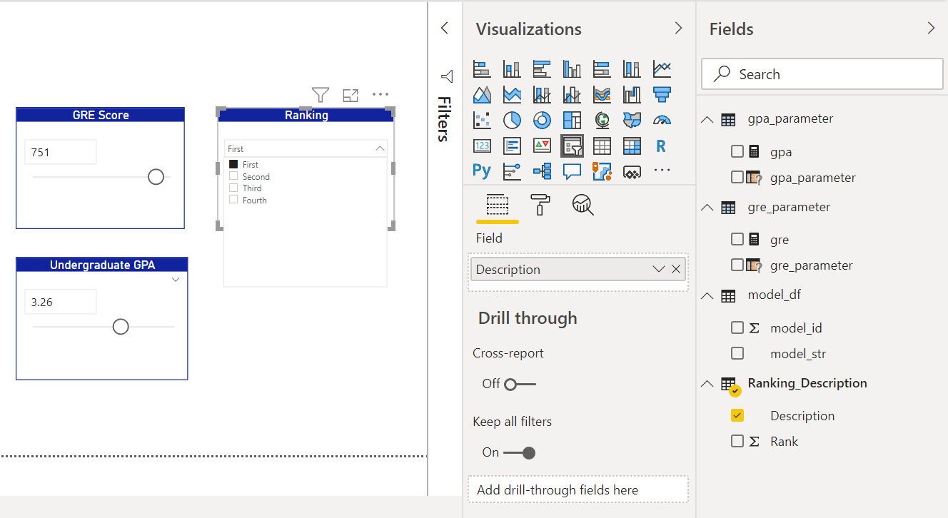
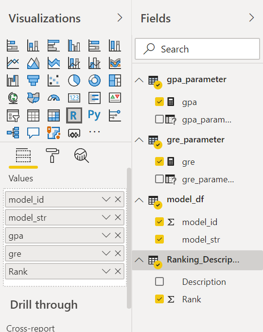
6. Now, we will tie it all together with the R-Script Visualization. Select the R visualization.
- In the R Visualization, for this example, we need the model_id, model_str, gpa measure, gre measure, and description (for rank). See below:
- In the ‘R script editor’ box, paste the following script:
from_byte_string = function(x) {
xcharvec = strsplit(x, " ")[[1]]
xhex = as.hexmode(xcharvec)
xraw = as.raw(xhex)
unserialize(xraw)
}
finalfit.str <- as.character(dataset[dataset$model_id == 1, "model_str"] )
finalfit <- from_byte_string(finalfit.str)
v <- c(gre = dataset$gre, gpa = dataset$gpa, rank = dataset$Rank)
pred <- round(predict(finalfit, newdata = as.data.frame(t(v))), digits = 2 )
plot.new()
text(0.5, 0.5,
labels = as.character(pred[[1]])
,cex = 3.5
)
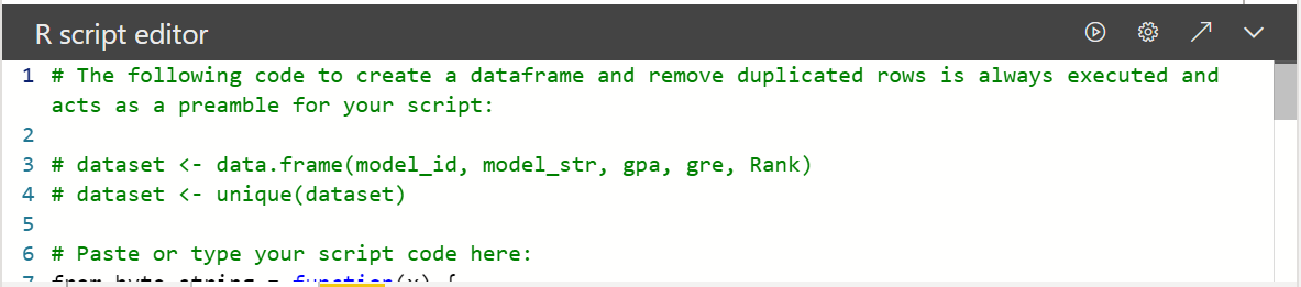
This code takes the string that was imported into model_df and reads it as the model that was originally created in R. It then takes the parameter values that appear on the slicer visualizations and uses them as the predictors in the model. Ensure that when you define the variables, they have the same naming convention that is used in the model built in R.
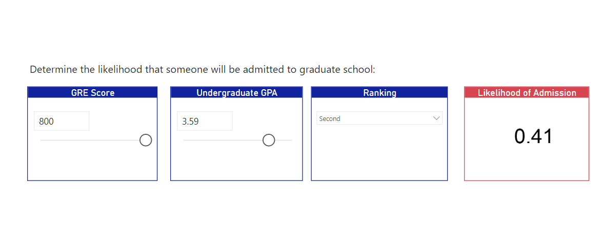
Once the slicers have been adjusted, the R-script visual should show the prediction, which inputs the values from the other 3 slicers into the model that was created in R and imported into Power BI. As the values of the variables are changed, the target variable changes as well.
This connection between R-studio models and Power BI allows for a technical user to create and display a model that they have tested and created. Then, it allows non-technical users to use the report and have hands-on access and insight into the predictive modeling and how variables will affect certain variables, such as sales or the likelihood of something happening.
For a copy of the .pbix file, please contact nicole.anderson2@rsmus.com.
If you have any questions about this process, advanced analytics, or Power BI in general, please visit our website, call 800-274-3978, or contact us.
RSM Staff
RSM empowers middle market companies worldwide to take charge of change. Our unique middle market perspective makes RSM the natural choice for growth-oriented, internationally active organizations seeking relevant insights and tailored, innovative solutions for a complex and changing world. With a global reach spanning more than 120 countries, we instill confidence in a world of change by bringing the full power of RSM to make a lasting impact on our clients, colleagues and communities.